CRM Experiment Lab — Segment-Stage Randomization, GCG and Net Effect
Situation
A CRM team ports product A/B habits into campaigns and breaks at randomization. Users are bucketed when they “show up” on launch day rather than when the campaign segment is built. Only part of the late arrivals reach the control arm, the arm shares diverge, and the sample-ratio-mismatch check fires on clean assignment.
The same mistakes repeat on every later layer: the global control group is refreshed by a full reshuffle and the comparison baseline jumps, the campaign effect is read without the price of unsubscribes, and the exposure window is sold as a free variance cut.
The lab puts all these layers into one synthetic experiment with a known answer, so each step can be checked and made to fail visibly.
Task
I needed a playground where the stages of a CRM experiment are checked against data whose true answer is known in advance, and where porting product logic produces a visibly wrong result rather than just a different number.
Actions
Simulator and the frozen data model
One run is 20,000 users, 28 days and 12 campaigns at seed 42. Five tables (users, campaigns, assignments, exposures, outcomes) are fixed by a contract before implementation, so the modules cannot quietly drift apart on the schema.
assignmentscarriesgroup ∈ {test, control, gcg}andstage ∈ {segment, exposure}, so the randomization stage is visible in the data;campaignscarriestrue_lift_ppandtrue_unsub_pp, the true effect of each campaign;outcomesgives purchases, purchase amount, unsubscribe and sessions per user-day.
Randomization: segment stage versus exposure stage
Two bucketing schemes are compared under the same assignment. Segment-stage bucketing keeps the fixed share and passes SRM; bucketing on first exposure drops late arrivals from control and inflates the test share.
| Stage | Test share | SRM p-value |
|---|---|---|
| segment (CRM-correct) | 0.4958 | 0.266 |
| first exposure (product-style) | 0.5629 | 0 |
Global control group
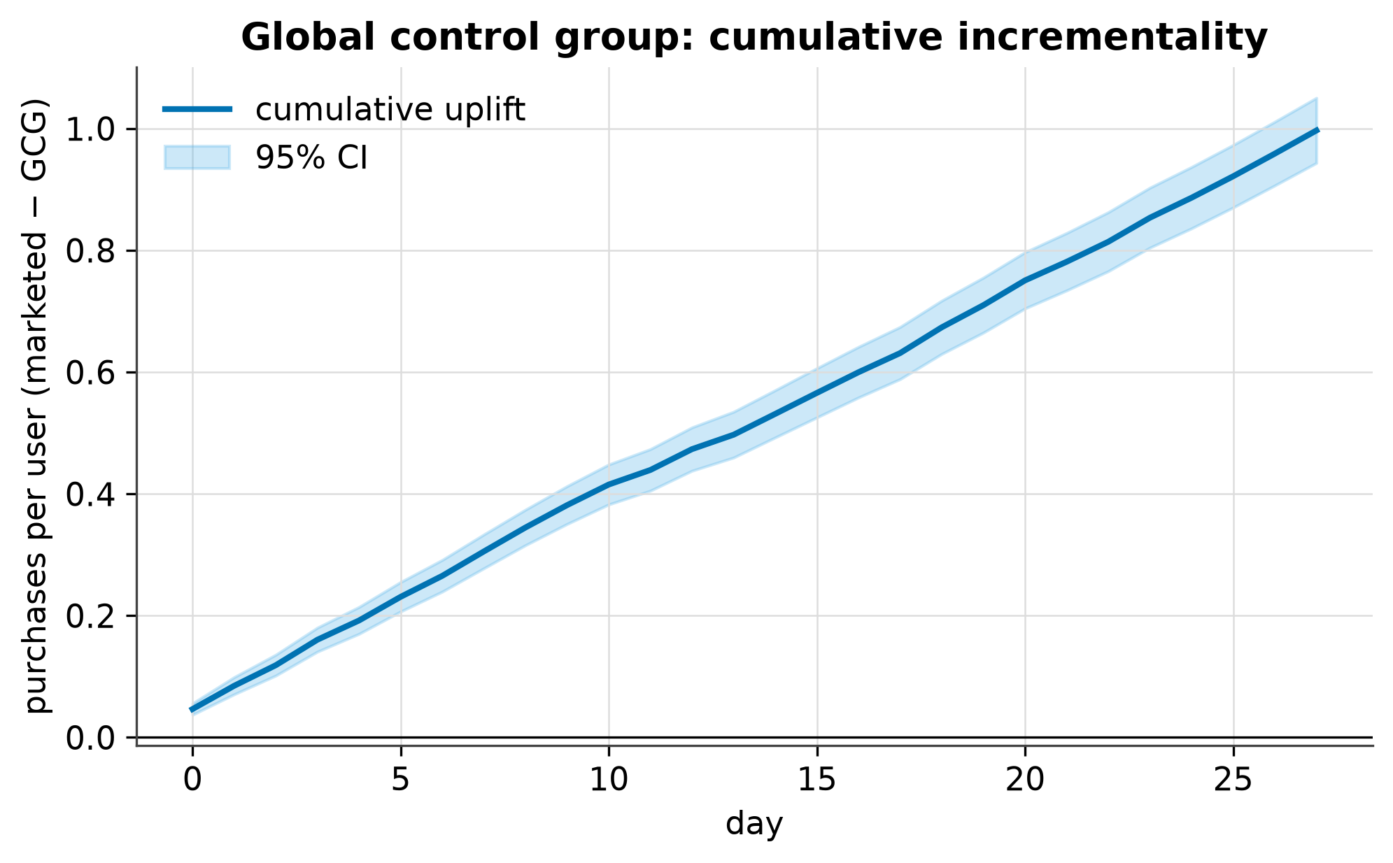
Uplift is “marketing minus global control”, so control stability is part of the estimate. A full reshuffle lifts the coefficient of variation of the trend to 0.3280; a partial rotation by config share keeps it at 0.0090.
Send balancer
The daily cap is three sends per user. The balancer spreads 12 campaigns across users and days, and no user-day exceeds the cap. Without it, send frequency grows with the number of campaigns and unsubscribes stop being a manageable cost.
Net effect with the price of unsubscribes
A campaign pays off only when incremental purchases outweigh incremental unsubscribes. Both sides are normalized per 1,000 treated users: +212.8 purchases against −162.3 unsubscribes, a net of +50.5 at a ratio of 1.311.
Exposure window and guardrails
The Is Exposed = True metric anchors both arms at the first exposure day. On a persistent effect that is a horizon anchor, not a standard-error cut; on a transient effect the effect-to-SE ratio rises from 7.55 to 12.28. The metric hierarchy — OEC (revenue), drivers, proxies, debug metrics and guardrails — is explicit so no single metric is optimized alone.
A/B readout
A separate report fixes the hypothesis, design and decision before the run: MDE 0.06765 absolute (10% relative), 751 users per arm, alpha 0.05, power 80%. SRM against the planned share: chi2=1.2395, p=0.2656. The cluster-robust standard error clustered by user matches the row-level one (1.00x), because the generator adds no within-user correlation.
Checks
A pytest suite of nine modules calibrates the statistics, the balancer, GCG, the exposure window and positivity; ruff holds the style. The pipeline runs in one command and rewrites the report and three figures.
uv sync --all-groups
uv run pytest
uv run python scripts/run_full_pipeline.py
Result
| Analysis | Result | Reading |
|---|---|---|
| Randomization (SRM) | segment p=0.266, exposure p=0 | the fixed share is balanced; activity bucketing is not |
| GCG uplift by day 27 | +0.9968 [0.9433, 1.0502] | the 95% interval excludes zero |
| GCG stability | full CV 0.3280 versus partial 0.0090 | partial rotation keeps the baseline steady |
| Net per 1,000 treated | +50.5 (212.8 − 162.3) | positive, ratio 1.311 |
| Exposure window | SE 0.00066 versus 0.00124 | the window anchors the horizon, it does not cut SE |
| Guardrails | 1 of 2 breached | unsubscribes fire, the daily cap holds |
The practical read is not “the campaign works” but “it works under an explicit churn budget”. The strict guardrail — unsubscribes must not rise — is unreachable at any send volume, because the treated arm is sent to and control is not. Under a 12% budget the send ships at cap 2, and the net maximum also lands at cap 2 (+56.8 per 1,000): fewer sends mean fewer unsubscribes, and the lost uplift is smaller than the churn saved. The readout verdict is Investigate, not Ship: the primary metric wins and the guardrail fails.
Limitations
The honest headline caveat: data/experiment_sample.csv is a 300-row outcomes-schema example with no group column, so the headline figures cannot be reproduced from it. Every number above comes from the simulator (scripts/run_full_pipeline.py), not from that CSV.
The data is synthetic and comes from a known generator: no interference between users, no bots, no delayed conversions, no logging loss, and the planted lift is constant in time. The GCG and exposure-window comparisons are estimators exercised on one seed, not a power study. There is no real assignment service, metric store or monitoring here: this is a single-experiment playground, not an experimentation platform.