← Back to portfolio A/B Testing Methodology Toolkit preview
Stack
PythonNumPy / SciPypytestuv
Impact
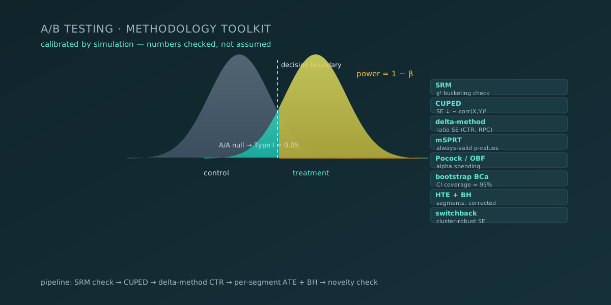
  • 15 modules, each calibrated by simulation: Type I error ≈ α, power curves
  • CUPED: SE shrinks by ~corr(X,Y)²
  • Naive peeking inflates Type I error — Pocock/OBF and mSPRT keep it under control
  • Delta method gives the correct SE for ratio metrics (CTR, RPC) — the naive per-unit t-test is biased
  • End-to-end pipeline: SRM → CUPED → delta-method CTR → per-segment ATE + BH → novelty check
Source View on GitHub → Updated: Sep 7, 2026

A/B Testing Methodology Toolkit

Context

An A/B testing method is only as good as its Type I error under the null and its power under a real effect. Rather than trusting asymptotic promises, each module simulates the pipeline end-to-end and reports the empirical rates.

Data & Method

Modules

Module Method What the demo shows
srm_test.py Sample Ratio Mismatch (χ²) catches bucketing/traffic bugs before any downstream test
sample_size.py Fixed-horizon sizing n/arm for proportions and means
delta_method_ratio.py Ratio metrics (CTR, RPC) correct SE for ΣY/ΣX; the naive per-unit t-test is biased
cuped.py Variance reduction SE shrinks by ~corr(X,Y)² using pre-period data
group_sequential.py Alpha-spending boundaries Pocock/OBF control Type I while naive peeking inflates it
msprt_always_valid.py Always-valid p-values mSPRT lets you peek and stop any time, validly
sequential_ratio.py Sequential ratio metrics delta-method + mSPRT for CTR under continuous monitoring
sequential_ab_testing.py Evan Miller’s sequential rule reproduces the size table, validates Type I/power, sample savings
bayesian_ab_test.py Analytic Bayesian A/B Beta-Binomial / Normal-Normal, P(B>A), expected loss, ROPE
bootstrap_ci.py Bootstrap CIs percentile & BCa for skewed metrics
heterogeneous_treatment_effects.py HTE by segment interaction model reveals Simpson-paradox-like cancellation
multiple_comparisons.py Multiple-testing correction Bonferroni (FWER) vs Benjamini-Hochberg (FDR)
novelty_primacy.py Time-varying effects treat×day interaction detects novelty decay / primacy growth
switchback.py Cluster & switchback designs cluster-robust SE; naive over-/under-rejects; carryover bias
test_simulator.py Generic test calibration plug any DGP + test → empirical Type I and power curve

End-to-end pipeline

scripts/run_full_pipeline.py ties the modules into one realistic flow on synthetic data: SRM check → CUPED → delta-method CTR test → per-segment ATE with BH correction → novelty check → a markdown report in outputs/report.md.

Testing Philosophy

The tests/ suite re-runs every calibration with assertions:

  • Type I error ≈ α (± tolerance) for each method under its null;
  • CI coverage ≈ 95% for the bootstrap;
  • naive peeking inflates Type I, always-valid / alpha-spending control it;
  • the naive per-unit ratio SE is inaccurate, the delta-method SE is accurate;
  • correctness on known-answer fixtures (SRM splits, segment uplifts, etc.).

Run

uv sync --all-groups
uv run pytest                 # calibration test suite
uv run python scripts/run_full_pipeline.py   # end-to-end demo → outputs/report.md

Impact

  • 15 calibrated modules — from SRM to switchback, each with an A/A null check.
  • Checked numbers — Type I ≈ α, coverage ≈ 95%, peeking controlled.
  • Unbiased ratio metrics — delta method instead of the naive per-unit t-test.
  • Cohesive pipeline — from SRM check to per-segment ATEs and a novelty check.

Documentation

Case study

Problem

A/B testing methods are sold on asymptotic promises, but nobody checks the Type I error under the null or the power under a real effect. Naive peeking, wrong SEs for ratio metrics, and multiple testing silently break decisions.

Approach

Each module is implemented from the primary literature and calibrated by simulation: an A/A null check for Type I error ≈ α and a power curve under a real effect. 15 topics are covered — SRM, sizing, CUPED, delta method, alpha spending (Pocock/OBF), mSPRT, sequential ratio, Bayesian A/B, bootstrap BCa, HTE, Bonferroni/BH, novelty/primacy, switchback. All wired into an end-to-end pipeline: SRM → CUPED → CTR test → per-segment ATE with BH → novelty check → report.

Result

The numbers are checked, not assumed: the test suite asserts Type I error ≈ α for every method, ≈95% CI coverage for bootstrap, peeking control for always-valid/alpha-spending, delta-method accuracy for ratio metrics, and correctness on known-answer fixtures.

15 Modules
A/A per method Type I error checks
~corr(X,Y)² SE reduction (CUPED)
Pocock/OBF, mSPRT Peeking control

Charts

Source: github.com/NikitaBoyarkin/ab_test: numbers re-produced by running scripts/group_sequential.py, scripts/msprt_always_valid.py, scripts/sequential_ab_testing.py and scripts/run_full_pipeline.py under `uv run python` (reproducible; plots/ and outputs/ are gitignored)

Type I error when peeking at interim looks

Empirical probability of a false positive across K=5 interim looks (40,000 null simulations). A naive z-test reapplied with a 1.96 boundary at every look, vs Pocock and O'Brien-Fleming boundaries calibrated to a total alpha of 5%.

0 5 10 15 Naive peeking — Type I error: 14.1 14.1 Pocock — Type I error: 4.9 4.9 OBF — Type I error: 4.9 4.9 Naive peeking Pocock OBF Design Empirical Type I error, %
Key takeaways
  • Rechecking with a 1.96 boundary at every one of 5 looks inflates the Type I error to 14.1% — nearly 3x the nominal 5%.
  • Alpha-spending restores control: both Pocock and OBF hold the error at 4.9%, at or below the nominal 5%.

False positives under continuous peeking

Probability of ever seeing p <= 0.05 across a stream t=1..500 under the null (2,000 streams). A standard z-test recomputed every step vs the always-valid mSPRT p-value (Johari et al. 2015), valid at any stopping time.

0 20 40 60 Naive z-test — False-positive rate: 47.8 47.8 mSPRT always-valid — False-positive rate: 3.2 3.2 Naive z-test mSPRT always-valid Method P(ever p <= 0.05), %
Key takeaways
  • Recomputing the naive z-test after every observation triggers a false positive in 47.8% of streams — nearly half of 'wins' are pure noise.
  • The mSPRT always-valid p-value cuts that risk to 3.2% — below the nominal 5% — while still letting you stop at any time.

Sequential test's average sample size

Evan Miller's sequential rule (N=808 successes, lead 56) vs a fixed horizon: the sequential test's average sample size as % of the fixed-sample size. 1,000 trials per case, 1% base rate, +20% MDE.

0 50 100 150 A/A (0%) — Avg sample size vs fixed: 118.6 118.6 A/B (+20%) — Avg sample size vs fixed: 76.3 76.3 Blockbuster (+40%) — Avg sample size vs fixed: 41.8 41.8 A/A (0%) A/B (+20%) Blockbuster (+40%) Trial type Avg sample size, % of fixed-horizon
Key takeaways
  • With a real +20% effect the sequential test finishes at 76.3% of the fixed-horizon sample on average, and at just 41.8% for a +40% effect.
  • Under the null (A/A) the sequential test spends 118.6% of the sample on average — savings appear only when a real effect exists.

Sample savings by minimum detectable effect

Sequential rule savings vs a fixed horizon at a 1% base rate (grid over MDE, 1,000 trials per point). Savings = (fixed-horizon expected successes - sequential average successes) / fixed.

0 5 10 15 20 Savings 0.1 — Savings: 20 0.2 — Savings: 14 0.5 — Savings: 1 0.1 0.2 0.5 Minimum detectable effect (relative) Sample savings, %
Key takeaways
  • At a 10% MDE the sequential test saves 20% of the sample, at 20% MDE it saves 14%, and at a 50% MDE savings drop to 1%.
  • Savings shrink monotonically with effect size, from 20% at a 10% MDE down to 1% at a 50% MDE — the rule pays off for small, long tests rather than for large effects.

See also

Connection map

Projects, posts and topics connected to this one. Hover a node to see its name; click to open.