SERP Rank Lab
▶ Data-flow diagram — self-contained HTML, opens in a browser — no install, no build
Situation
A metasearch site sells no tickets. Its revenue is a partner commission or a cost-per-click, multiplied by which position the offer occupied on the results page. So the role rests on two questions: how to rank offers, and how much revenue a given ranking policy produces per search.
The offline relevance metric and the money disagree: a policy that looks better on NDCG can earn less commission.
Task
I needed to build the measurement substrate for that surface — an unbiased (position-free) CTR, ranking metrics, and an A/B readout over the ranking policy — and tie them into one reproducible pipeline.
Actions
Layers
| Layer | Files | Role |
|---|---|---|
| Data | src/data_ingest.py, sql/01_normalize.sql |
booking feed → one row per leg; orders and events normalisation |
| Sessions | src/sessions.py, sql/02_sessions.sql |
30-minute inactivity + date-boundary session rule |
| SERP | src/serp_sim.py |
synthetic pages over real route/price pairs; PBM click model; CPA/CPC economics |
| Evaluation | src/ranking_eval.py, sql/03_funnel.sql, sql/04_revenue_per_search.sql |
unbiased CTR, NDCG/MRR, interleaving, revenue per search |
| Experiment | src/stats.py, src/experiment.py |
SRM, A/A, delta method, CUPED, mSPRT, peeking |
| Surface | app.py, run.py |
Streamlit dashboard; single pipeline entry point |
Methods
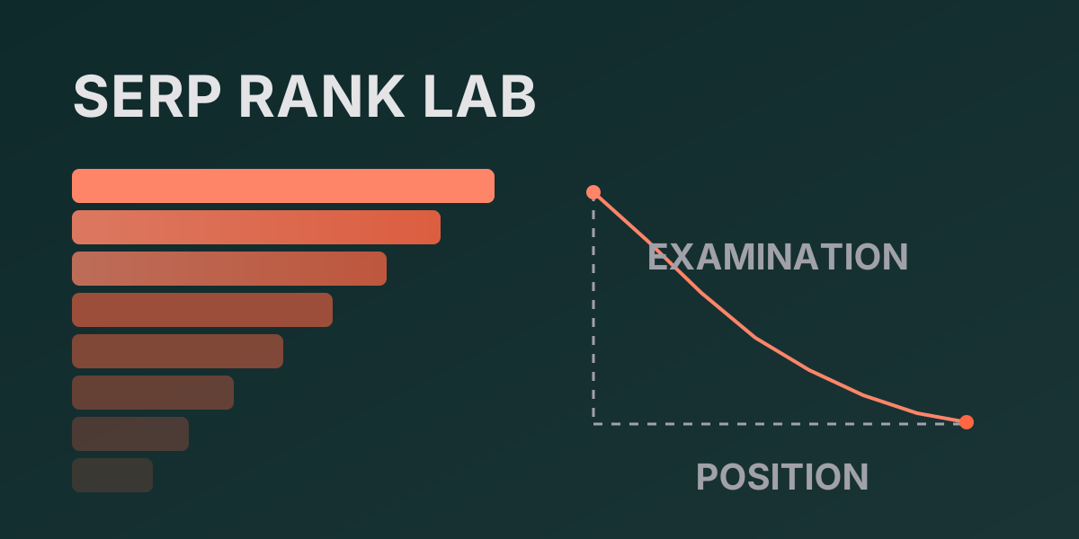
- Position bias (PBM). Examination probability decays with position as
(1/k)^η; a click is examined × relevance. - Unbiased CTR. Horvitz–Thompson inverse-propensity weighting, with the curve known or fitted by EM.
- Ratio metrics. Revenue per search is a ratio of sums, so its variance comes from the delta method, not a naive per-unit t-test.
- Sequential testing. A fixed horizon against an always-valid mSPRT to quantify the peeking penalty.
Run
uv sync --all-groups
uv run python run.py --stage all      # ingest → sessions → serp → sql → rank → experiment → business
uv run pytest -q                      # 110 tests (108 pass, 2 skip without sibling data)
uv run streamlit run app.py           # dashboard on :8501
Result
| Check | Result | Reading |
|---|---|---|
| NDCG@10 vs revenue/search | relevance-first: 1.000 / 869.5, revenue-first: 0.931 / 1,193.7 | the policies move in opposite directions — revenue 38% higher |
| Naive vs position-free CTR | 0.163 vs 0.629 | understated roughly fourfold |
| SRM vs the planned 90/10 | χ² = 0.119, p = 0.730 | the split is sound |
| Ratio metric, delta method vs naive | SE 69.0 vs 88.5 | the naive SE is 1.28× too wide |
| Peeking, fixed horizon | FPR 14.5% over ten looks | 2.9× the nominal rate |
| Peeking, mSPRT | FPR 0.25% | the always-valid threshold holds the level |
The pipeline runs end-to-end from a fixed seed; 108 tests pass, 2 skip without the optional sibling data.
Limitations
The synthetic SERP layer resembling real traffic is an inference — no real impression log exists for this surface, so every ranking and A/B number comes from a model, not a measurement. Two islands of real data (orders and booking legs) carry no foreign key to the clickstream and are reported separately, never fused with the modeled SERP metrics. Raw third-party data is not committed: the repository holds only the loader, the SERP generator and the SQL.
Documentation
Frequently asked
Why is the offline ranking metric a bad release gate?
The policy that maximises NDCG@10 collects more clicks but earns 38% less per search than revenue-first. The north star has to be revenue per search, not an offline relevance score.
How biased is the naive CTR?
Fourfold: 0.163 against a position-free 0.629. The cause is position bias, not the metric itself, and inverse-propensity weighting fixes it.
Why is repeated peeking dangerous?
On a fixed horizon the false-positive rate climbs to 14.5% over ten looks. Always-valid mSPRT holds it at 0.25%, at the price of a wider threshold.
What does the 90/10 split cost?
2.78× the traffic of a 50/50 split for the same power: 55,196 versus 19,871 users.
What did CUPED show on real data?
On i.i.d. users the covariate buys nothing (correlation near zero), while on a correlated positive control it recovers the theoretical 11.2% variance cut.