Delivery Control Tower
Situation
Delivery is usually measured as one number — the average time. That is not enough to see where the process loses time: the split by category, channel and city shows different causes, and an order forecast is needed to plan capacity in advance.
Task
I had to build a reproducible analytics loop: land the data in marts, verify it with named quality checks, produce a forecast and compare it honestly with a baseline, locate the bottlenecks, test pre-registered hypotheses, and show a SQL layer with measured optimizations.
Actions
Data and marts
The source is the aggregate table from a public data-analyst test task (Dodo Brands): 550,710 rows of day × city × channel × category for 2022-01-01..2022-06-30, 264 cities, 3 channels, 4 categories. A second file is a sample of 130,079 orders across 2 anonymized cities, used for the SQL layer only.
The ETL moves raw → staging parquet, quality.py checks row counts, grain uniqueness and ranges, and marts.py builds a DuckDB star schema: six dimensions, two fact tables and three marts. tickets means orders (33,167,293), qty means items (57,576,550), 1.736 items per order.
Forecast
Rolling-origin backtest: a 28-day test window, four folds, refit every 7 days. Four models at horizons 1/7/14. Features for day t are built only from observations strictly before t.
| Model | h=1 | h=7 | h=14 |
|---|---|---|---|
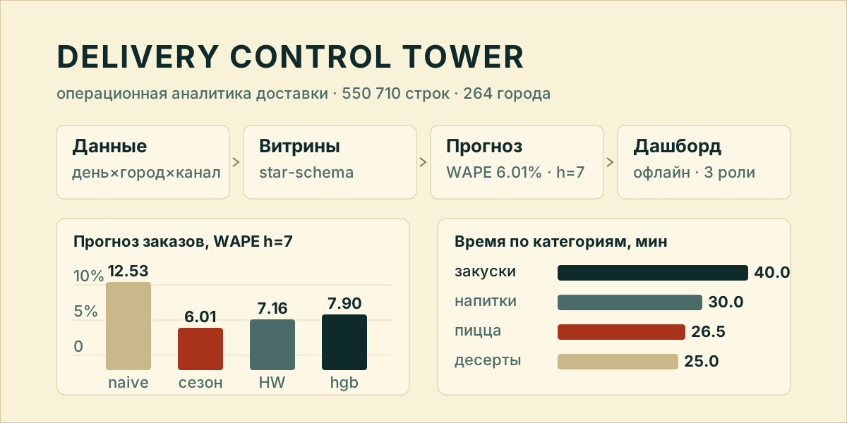
| naive | 22.68 | 12.53 | 12.54 |
| seasonal_naive | 5.40 | 6.01 | 6.25 |
| holt_winters | 3.91 | 7.16 | 7.22 |
| hgb | 7.14 | 7.90 | 8.09 |
Bottlenecks
Three views on one question. The channel × category decomposition: snacks ≈40.0 min, pizza ≈26.5 min, drinks ≈30.0 min, desserts ≈25.0 min; the channel moves time by tenths of a minute. The load curve: mean time per volume decile falls from 31.88 to 31.24 min, rho = −0.092. City ranking by the avg_time ~ qty slope: the top is Усолье-Сибирское (index 2.02), Грозный (1.63), Магадан (1.18), but slope R² is 0.0004–0.0185 — a prioritization aid, not a proven trend.
Hypotheses
| Hypothesis | Effect | p | 95% CI | Verdict |
|---|---|---|---|---|
| H1: mp share grows faster than web | +5.70 pp | 2.07e-11 | [5.35; 6.03] | supported |
| H2: weekends are slower than weekdays | −0.93% | 1.1e-41 | [−1.09; −0.76] | rejected: significant effect in the opposite direction |
SQL and presentation
sql/windows.sql holds 14 named window queries: moving averages, weekly growth, ranks, Pareto, 3×MA7 anomalies, gaps between a client’s orders. Three slow/fast pairs under EXPLAIN ANALYZE: 5.66×, 3.23× and 1.27×; the best is a running order count over 130,079 rows (62.3 → 11.0 ms).
The dashboard is a single offline HTML file of ≈81 KB with no CDN and no client-side requests, split into three role blocks: operations, commerce, leadership. The Superset recipe in superset/ is written but was never started: Docker is unavailable on the build machine, and the README says so instead of hiding it.
Result
The forecast reaches 6.01% WAPE at the weekly horizon (h=7) with the seasonal baseline; the complex model does not beat it, and that is what the recommendation says. The bottleneck is category, not load (rho = −0.092): snacks take 40.0 min against 26.6 min for pizza, 13.4 min (+50%) longer in every channel. The channel mix is shifting: the mp share grew 5.7 pp in six months. One negative result — H2 on weekends — was rejected by the pre-registered rule: the effect is significant but in the opposite direction.
Limitations
The data is aggregated to day × city × channel × category: there is no per-order, courier or restaurant timing. cost is a money metric with unconfirmed currency, and avg_price does not reconcile with it and is not used. The order sample covers two anonymized cities. The backtest has four folds, so differences of a few hundredths of a point are not meaningful. Nothing here is causal: the tests are associational.
Documentation
README.md covers architecture, quickstart and limitations; reports/report.md is the analytical report; docs/data_dictionary.md is the field dictionary.
Frequently asked
Why does delivery time not depend on load?
On the day × city × channel × category aggregate the Spearman correlation between volume and time is rho = −0.092, and mean time moves from 31.88 to 31.24 min across extreme deciles. The spread is explained by category, not by order count.
Which forecast model was chosen?
For 7- and 14-day horizons, seasonal_naive: WAPE 6.01% and 6.25%. Holt-Winters wins only one day ahead (3.91%), and gradient boosting beats the seasonal baseline at no horizon.
Which field must not be read as revenue?
The cost field is a money metric in unconfirmed source units: its currency is undocumented. avg_price does not reconcile with cost (221.8 vs 138.9) and is not used in any calculation.